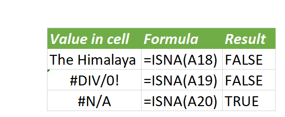
The ISNA() function could be a logical function that returns the value in True / False. It checks whether or not the argument is #N/A error or not. It keeps one parameter that’s a value.
Where to use :
ISNA() operate is extremely helpful to manage #N/A error value over excel sheets.
Syntax :
=ISNA(value)
Parameters :
Value – value suggest that any information or a cell reference.
When this error comes.
This error comes once a value that you are searching for isn’t found within the item list. If the value isn’t found, it reflects #N/A. This error particularly found as an outcome of lookup functions like Vlookup, Hookup, Offset, Match etc.
Example-:
Now understand however you’ll get rid of the #N/A error in Microsoft excel – let’s check the below example
Example : we have two information sets within which we want to populate the Joining date from the first data set into the second data set 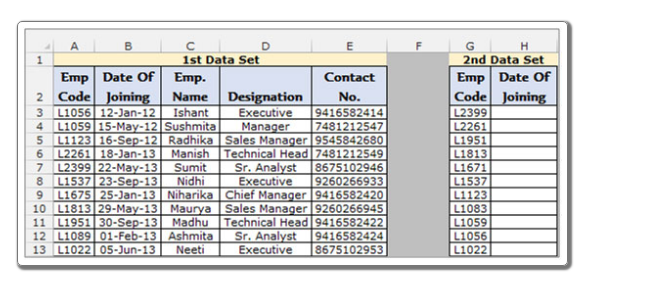
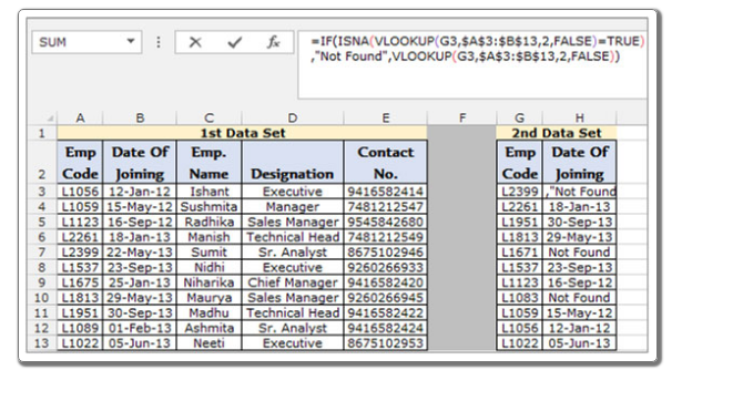
Pick the Cell H3, & write the formula.
=IF(ISNA(VLOOKUP(G3,$A$3:$B$13,2,FALSE)=TRUE),”Not Found”, VLOOKUP(G3,$A$3:$B$13,2,FALSE))
The function will return the joining date of employee.
Copy the formula to the other cells to return the joining date for all row populated in column A.
To Copy the formula in all cells press key “CTRL + C” in cell H3 and choose the cellsH4 to H13 and press key “CTRL + V” on the keyboard.
The employee codes which are exist in the 2nd data set but not exist in the 1st data set will show the “Not Found” result in place of the #N/A error.
To accomplish, you can use this formula if you need the formula to show some text instead of the #N/A or any such error. You can even ask the formula to return blank cells by changing the “Not Found” with”.