Constraints in linear programming

Decision variables are used as mathematical symbols representing levels of activity of a firm. Parameters are the numerical coefficients and constants used in the objective function and constraint equations. Likewise, constraints are restrictions placed on the firm by the operating environment stated in linear relationships of the decision variables. Constraints illustrate all the possible values that the variables of a linear programming problem may require. They typically represent resource constraints, or the minimum or maximum level as explained below:

Assume: X₁, X₂, X₃, ………, X_n to be decision variables of an activity

Z = Objective function or linear function

Requirement: Maximization of the linear function Z.

Z = c₁X₁ + c₂X₂ + c₃X₃ + ………+ c_nX_n …..Eq (1)

subject to the following constraints:

a₁₁x₁ + a₁₂x₂ + … + a_1nx_n (≤, =, ≥) b₁

a₂₁x₁ + a₂₂x₂ + … + a_2nx_n (≤, =, ≥) b₂

:

a_m1x1 + a_m2x₂ + … + a_mnx_n (≤, =, ≥) b_m

In this case, a_ij, b_i, and c_j are given constants where:

x_j = decision variables

b_i = constraint levels

c_j= objective function coefficients

a_ij = constraint coefficients

1. the function Z is the objective function.
2. x₁, x₂, . . . ,x_n are the decision variables.
3. the expression (≤, =, ≥) means that each constraint may take any one of the three signs.
4. c_j (j = 1, . . . , n) represents the per unit cost or profit to the j th variable.
5. b_i (i = 1, . . . , m) is the availability of the ith constraint.
6. x₁ , x₂ , . . . , x_n ≥ 0 is the set of non-negative restriction on the linear function.

Resource constraints are accepted as the common type of constraint wherein the coefficient aj,i indicates the amount of resource j that is needed for each unit of activity i, shown by the value of the variable Xi. The RHS of the constraint (bj )shows the total amount of resource j that is available for the activity. The constraint above can be written as a using both ≤ ,≥ inequalities. A greater-than-or-equal constraint is converted to a less-than-or-equal by factoring X-1. Similarly, equality constraints can be written as two inequalities — a less-than-or-equal constraint and a greater-than-or-equal constraint.

The variables of linear programs must always take non-negative values which means that the values are greater than or equal to zero). The variables can show the levels of a set of activities or the amounts of some resources used. Such a non-negativity requirement will be reasonable and even necessary. In the rare case where you want to allow a variable to take on a negative value, there are certain formulation “tricks” that can be employed. These “tricks” also are beyond the scope of this class, however, and all the variables we will use will only need to take on non-negative values.

Example: How many bowls and mugs should be produced to maximize profits given labour and materials constraints?

Product resource requirements and unit profit:

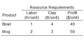
Resource 40 hrs of labor per day

Availability: 120 lbs of clay

Decision Variables x₁ = number of bowls to produce per day and x₂ = number of mugs to produce per day

Objective Maximize Z = $40x₁ + $50x₂

Function: Where Z = profit per day

Resource 1x₁ + 2x₂ 40 h labor

Constraints: 4x₁ + 3x₂ 120 lbs clay

Non-Negativity Constraints: x₁ 0; x₂ 0

Complete Linear Programming Model:

Maximize Z = $40x₁ + $50x₂

subject to: 1x₁ + 2x_{2 ≤} 40

4x₁ + 3x_{2  ≤} 120

x₁, x_{2  ≥} 0