Optimal feasible solutions (up to three non-trivial constraints)
A feasible point on the optimal objective function line for an LP provides an acceptable optimal solution.The following Theorems are fundamental in solving linear programming problems to obtain an optimal solution:
Theorem 1
When you consider R to be in the feasible region (convex polygon) and let Z = ax + by be the objective function. Then, Z contains an optimal value (maximum or minimum), with the variables x and y that are subject to constraints described by linear inequalities. This optimal value must be spotted at a corner point (vertex) of the feasible region.
Theorem 2
When you consider R to be the feasible region and let Z = ax + by be the objective function. If R is bounded, then the objective function Z obtains the max and min values on R which occurs at a corner point (vertex) of R.
Example: Maximize Z = $40x1 + $50x2
subject to: 1x1 + 2x2 40
4x2 + 3x2 120
x1, x2 0
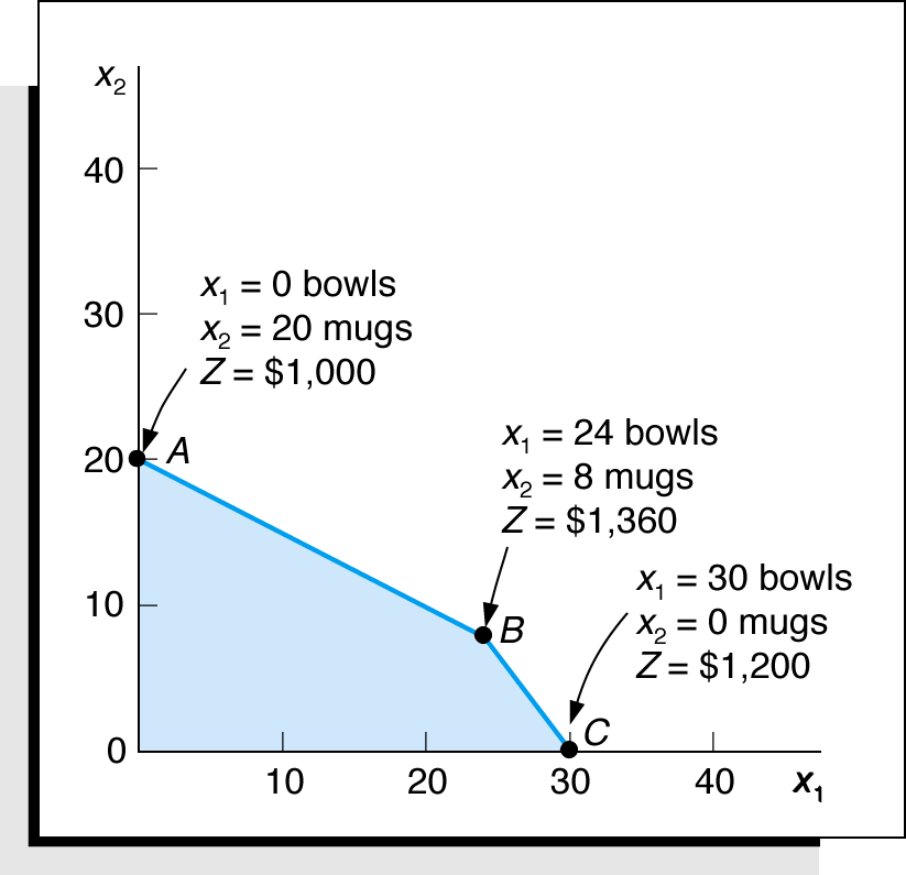
Figure 1: Solutions at all the corner points |
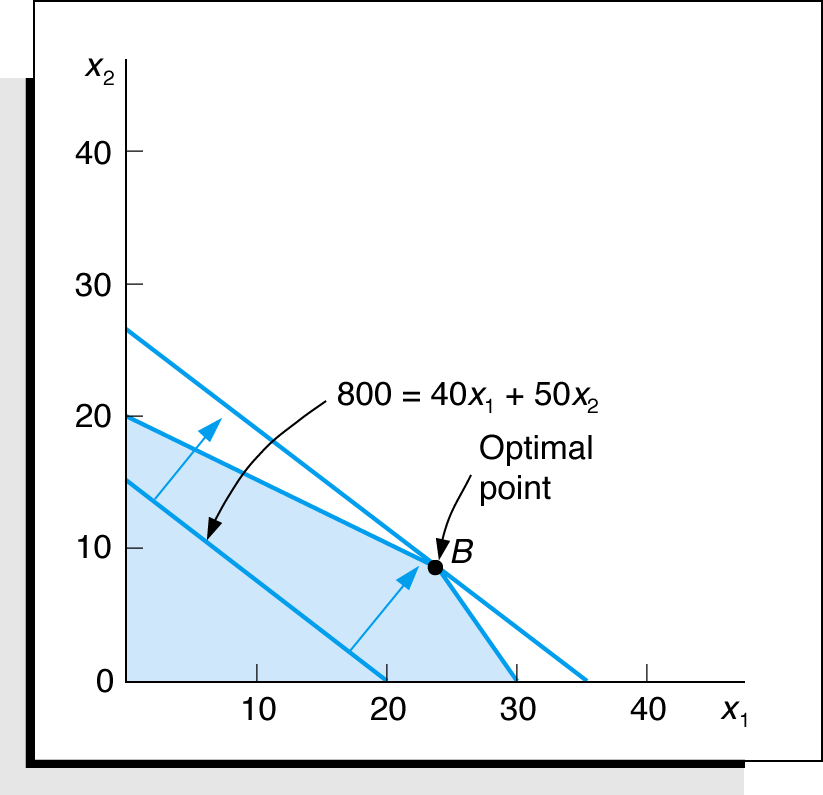
Figure 2: identification of optimal point. |
Now let objective function for the above example be different while the constraints remain same:
Maximize Z = $70x1 + $20x2
subject to: 1x1 + 2x2 40
4x2 + 3x2 120
x1, x2 0
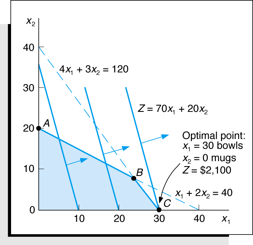
Figure 3: Optimal Solution with Z = 70x1 + 20x2
As shown in the graph above, an LP problem may have more than one optimal solution. Graphically, when the profit (or cost) line runs parallel to a constraint in the problem which lies in the direction in which profit (or cost) line is located.
Example: Maximize profit = $3x + $2y
Subject to:
6X + 4Y 24
X 3
X, Y 0
In this case, The objective function is parallel to a constraint line.
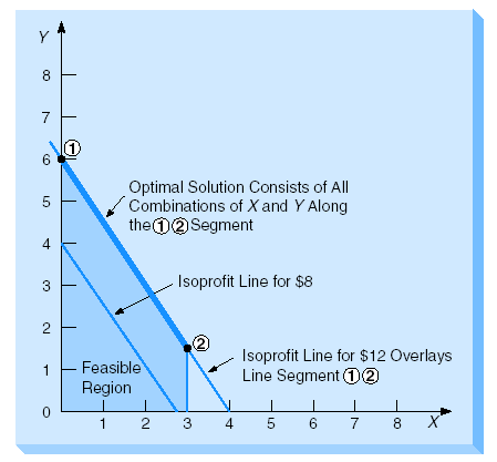
At the profit level of $12, profit line will rest directly on top of the first constraint line.Hence, any point along the line between corner points denoted 1 and 2 provides an optimal X and Y combination. Notice that in the figure above the objective function is parallel to one of the edges of the feasible region. We can consider that any point along this edge between the two extreme points contains the optimal solution which maximizes the objective function. In this case, there is no unique solution, but there is an infinite number of optimal solutions.