We have previously discussed word-problems translated into mathematical problems in the form of linear programs.The graphical method is applicable to solve the LPP involving two decision variables x1, and x2, however, more number of variables are difficult to optimize by graphical representation.The solution is a set of values for each variable:
- are consistent with the constraints (i.e., feasible), and
- produce the best possible value of the objective function (i.e., optimal).
Not all LP problems have a solution, however. There are two other possibilities:
- there may be no feasible solutions (i.e., there are no solutions that are consistent with all the constraints), or
- the problem may be unbounded (i.e., the optimal solution is infinitely large).
If the first of these problems occurs, one or more of the constraints will have to be relaxed. If the problem is unbounded then the problem probably has not been well formulated since few, if any, real-world problems are truly unbounded.The graphical representation and solution of an LP problem aids in understanding more intuitively what an LP is and how it is solved.
Graphical solution method:
Draw the 1st quadrant graph: x-y plane since the two decision variable x and y are non-negative
Plot model constraint lines and planes on a set of coordinates in a plane. The first constraint inequality divides the first quadrant into two regions say R1 and R2, suppose (x1, 0) is a point in R1. If this point satisfies the in equation ax + by ≤ c or (≥ c), then shade the region R1. If the point (x1, 0) does not satisfy the inequality, then shade the region R2.
Now identify the feasible solution space on the graph where all constraints are satisfied at the same instance
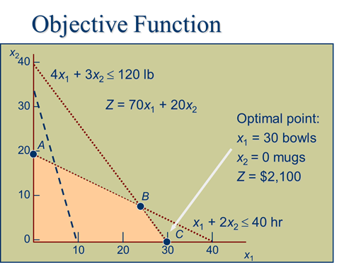
Plot objective function to find the point on the boundary of this space that maximizes (or minimizes) value of the objective function
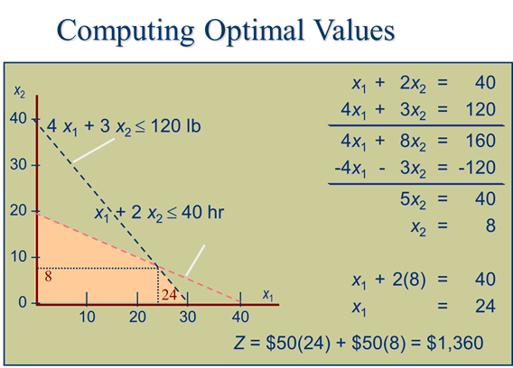
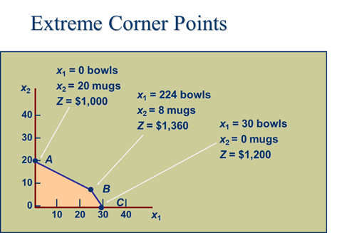
Compute the optimum solution by finding a corner point.
The intersection of both the region from the inequalities shows the feasible solution of the LPP. Therefore every point in the shaded regionis a feasible solution of the LPP as this point agrees with all the constraints including the non-negative constraints.
These coordinates are provided from the graph or by solving the equation of the lines.
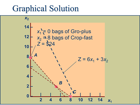
Consider a minimization problem:
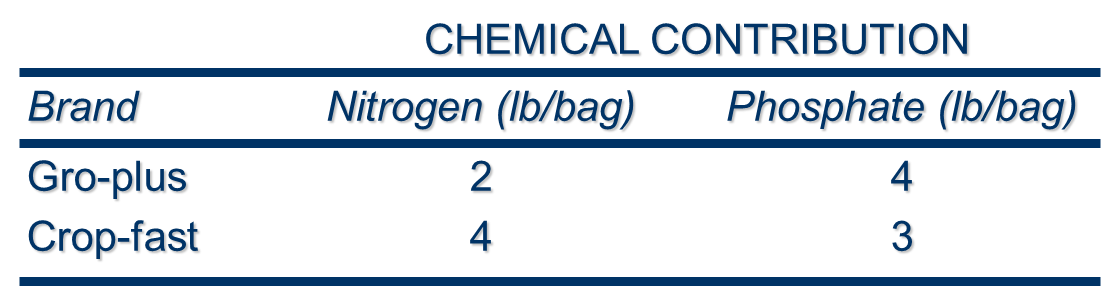
Minimize Z = $6x1 + $3x2
subject to
2x1 + 4x2 16 lb of nitrogen
4x1 + 3x2 24 lb of phosphate
x1, x2 0